Tutorial

Getting Started

Getting started with binmod1d is simple. Users will first initialize the spectral model using the spectral_1d() class:

from binmod1d.spectral_model import spectral_1d

s1 = spectral_1d()

The inputs to this class will specify the initial gamma particle size (or mass) distribution (PSD), the bin resolution (sbin) and number of bins used (bins), as well as other parameters that determine how the model will be run.

In general, the most relevant inputs are:

• sbin int
  Resolution of geometric mass bins (default: 2).

• bins int
  Number of mass bins for the distribution (default: 60).

• dt float
  Model time step in seconds. (default:1)

• tmax float
  Maximum time in seconds the model is run (default: 800).

• output_freq int
  Frequency in with which the model is output. (default: 1)

• dz float
  Height grid spacing in meters. (default: 20.)

• ztop float
  Top height of steady-state/1D model domain in meters. (default: 0.)

• zbot float
  Bottom height of steady-state/1D model domain in meters. (default: 0.)

• D1 float
  Minimum equivolume diameter bin size in mm when the dist_var parameter is ‘size’. (default: 0.1)

• x0 float
  Minimum bin mass in grams when the ‘dist_var’ parameter is ‘mass’. (default: 0.01)

• moments int
  Number of moments to use for spectral bin model (either 1 (mass) or 2 (mass and number)). (default: 2)

• dist_var str
  Whether to use mass or size to specify initial gamma distribution. (default: ‘size’)

• kernel str
  Type of collision kernel in collection_kernels.py to use for coalescence/breakup. (default: ‘Hydro’)

• frag_dist str
  Type of fragment distribution. (default: ‘LGN’)

• ptype str
  Whether particles are rain or snow. (default: ‘rain’)

• habit_params str/list/dict
  Name(s) of habit parameters used for each distribution category. Multiple categories are included if input is a list of strings (default dictionaries) or dictionaries. (default: ‘rain’)

• Ecol float
  Collision efficiency. (default: 1.0)

• Es float
  Sticking/coalescence efficiency. (default: 1.0)

• Eb float
  Breakup efficiency. (default: 0.0)

• wavl float
  Radar wavelength in millimeters. (default: 110.0)

• radar bool
  Whether to compute radar variables. (default: False)

• cc_dest int
  Distribution destination from 1 to len(habit_params) for coalesced particles. (default: 1)

• br_dest int
  Distribution destination from 1 to len(habit_params) for breakup/fragmented particles. (default: 1)

• rk_order int
  Runge-kutta order with options of orders 1 through 4. (default: 1)

After the model is initialized, users can then use the run() method to run the model with the inputs specified in spectral_1D:

s1.run()

Various methods are included in the spectral_1d.py class that allow for easy plotting of bin model setup and results. For example, after the spectral_1d() object is initialized, users can view the initial number and mass distributions using the plot_init() method.

s1.plot_init()

The following plotting methods are include:

spectral_1d.plot_init()

Plots the starting number and mass binned distribution.

spectral_1d.plot_dists()

Plots the resulting number and mass distributions at a particular time and height.

spectral_1d.plot_dists_height()

(steady-state and full 1D model only) Plots the resulting number distributions at a particular time for a range of heights.

spectral_1d.plot_moments_radar()

(steady-state/full 1D modes) Plots height profiles of number concentration, mean volume diameter, water contents, precipitation rates, and radar variables. Box model mode instead plots timeseries of each variable.

spectral_1d.plot_time_height()

(full 1D model only) Plots the time/height pcolor profiles for a particular microphysical or radar variable.

📏 Units & Conventions

BinMod1D primarily uses CGS units for internal calculations (cm, g, s). However, for user convenience, inputs usually follow these conventions:

Quantity	Unit	Parameter Examples
Size	millimeters (mm)	Dm0, D1
Mass	grams (g)	x0, Mbins
Height	meters (m)	dz, ztop, zbot
Total Number	per liter (\(L^{-1}\))	Nt0
Bin Number	m\(^{-3}\)	Nbins

Note: This prevents the need for very large or small scientific notation for typical rain/snow cases.

Illustrative Examples

Here, I’ll use the same type of simulation (i.e., continental rain) with the same initial gamma distribution but run in different ways. Let’s assume also that users have a particular set of predetermined gamma size distribution parameters that govern and initial size distribution. Often, researchers tend to (unwisely) use the \(N_{0}\), \(\Lambda\), \(\mu\) convention where the gamma distribution is defined as

\[ n(D) = N_{0} D^{\mu} \exp(-\Lambda D). \]

Of course, when parameterized in this way, it is generally difficult at a glance to get a sense for how these distribution parameters correlate to key properties like the total number and mean sizes of the initial population of particles. Therefore, the initial gamma distribution input is instead parameterized as

\[ n_{0}(D) = 1000\, \frac{N_{t,0}}{\Gamma(\mu_{0}+1)} \frac{1}{D_{m,0}} \left( \mu_{0}+4 \right)^{\mu_{0}+1} \left( \frac{D}{D_{m,0}}\right)^{\mu_{0}} \exp\left[ - (\mu_{0}+4) \frac{D}{D_{m,0}}\right], \]

where \(n_{0}(D)\) has units of m\(^{-3}\) mm\(^{-1}\) and

\[ \begin{align}\begin{aligned} N_{t,0} = N_{0} \Lambda_{0}^{-(\mu_{0}+1)}\, \Gamma(\mu_{0}+1)\\D_{m,0} = \frac{\mu_{0}+4}{\Lambda_{0}}\\\mu_{0} = \mu_{0}.\end{aligned}\end{align} \]

Here, \(N_{t,0}\) is the initial total number concentration of the distribution whereas \(D_{m,0}\) is the initial mean volume diameter which is defined as

\[ D_{m} \equiv \frac{M_{4}}{M_{3}} = \frac{\int\limits_{D=0}^{\infty} D^{4} n(D) dD}{\int\limits_{D=0}^{\infty} D^{3} n(D) dD}. \]

In this tutorial, let’s start with a rain distribution with the following parameters: \(N_{t,0}=10\, \mathrm{L}^{-1}\), \(D_{m,0}=1.25\, \mathrm{mm}\), and \(\mu_{0}=0\) (i.e., an exponential or Marshall-Palmer distribution) and then evolve these distributions in each mode.

Box model mode

First, let’s set up a box model run. To do this, we need to first determine the grid we’ll be using by using the D1 size parameter which specifies the initial left edge of the first size distribution bin. Because we are determining the grid parameters based on size, we also need to set the dist_var parameter to ‘size’ rather than ‘mass’. Finally, we use the dt and tmax parameter to specify the timestep and the maximum time we want to go out to. Finally, we can set the output_freq parameter to 1 to let the model know that we want the final distribution arrays to be for all timesteps (for more involved and computionally heavy model runs, users can set this parameter to a higher value). Let’s also specify that we want a collision efficiency \(E_{\mathrm{col}}\) of unity and a coalescence efficiency of \(0.2\) and that we want the hydrodynamic kernel. We’ll also run the model out to 30 minutes to get a nice timeseries when we plot some results.

rain_box = spectral_1d(sbin=2,bins=60,D1=0.01,dt=2.,tmax=1800.,Nt0=10.,Dm0=1.25,mu0=0.,habit_params=['rain'],ptype='rain',kernel='Hydro',Ecol=1.0,Es=0.2,radar=True,dist_var='size')
rain_box.run()

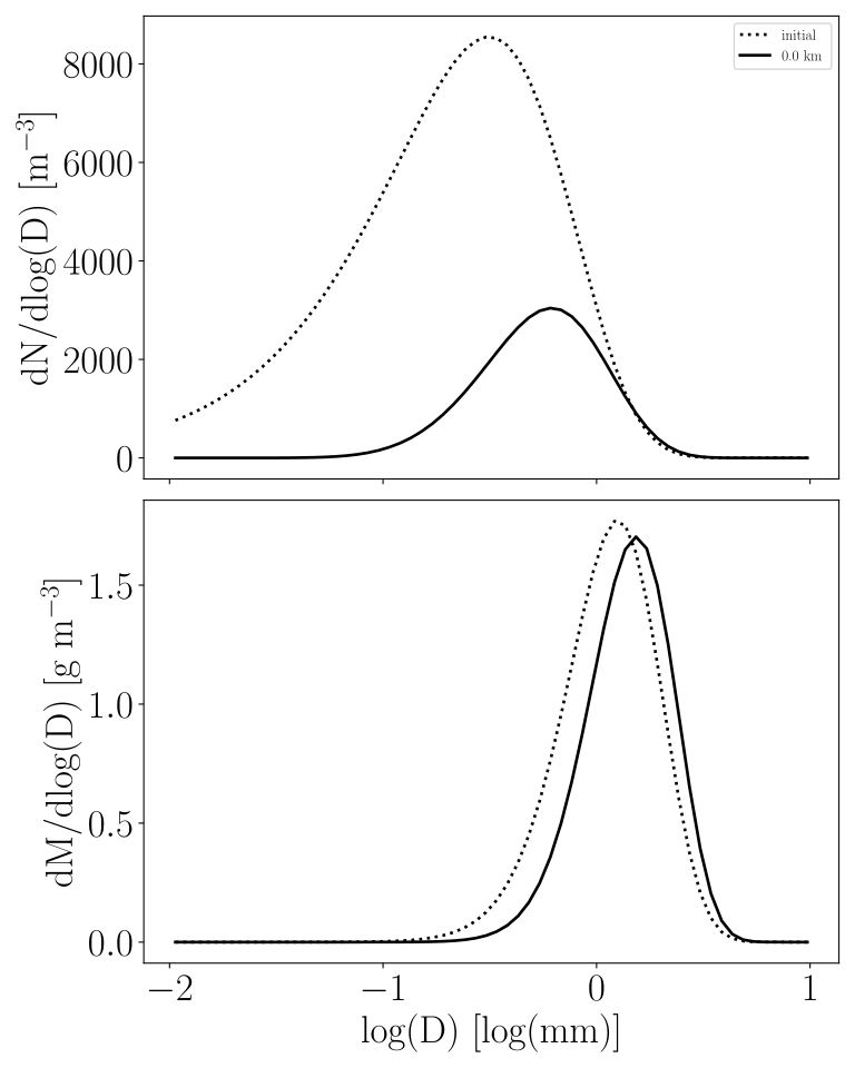
This run should be really quick for an sbin value of 1 and only one distribution. Now let’s look at the results. First, let’s use the plot_dists() method to plot the initial and final number and mass distribution functions

rain_box.plot_dists(x_axis='size')

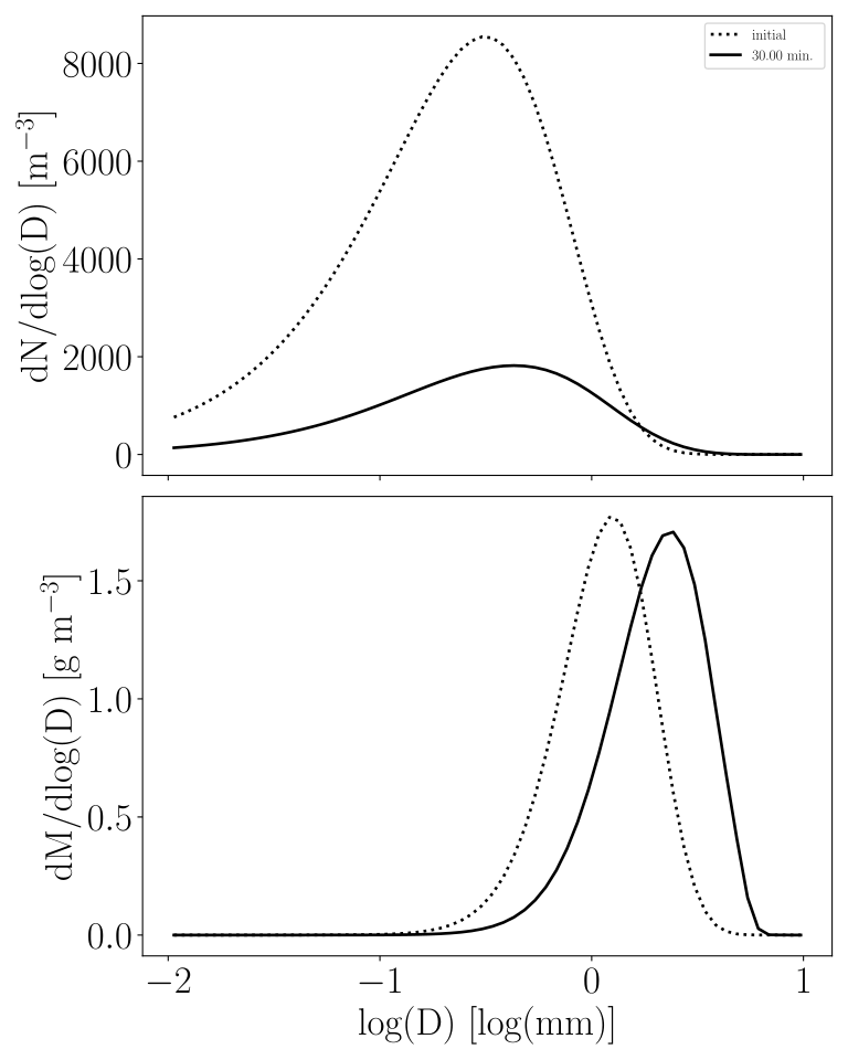
Notice that with collision-coalescence on, the number and mass distributions shift toward larger sizes from the initial time to \(30\) minutes. The default plotting for plot_dists() is in terms of \(dN/d\log(D)\) and \(dM/d\log(D)\) (i.e., distscale='log') because this reliably produces nice bell-shaped distributions. However, we can use some of the optional input parameters to customize the plots a bit more in the style of what are typically shown in journal articles. 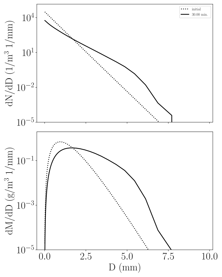Often, researchers will plot these distributions in a semi-log fashion where the \(x\)-axis is linearly spaced but the \(y\)-axis is log-spaced. Exponential distributions (like our initial Marshall-Palmer one) will appear as straight lines in the number distribution plots when plotted in this way. We can reproduce the number and mass distribution plots in a semi-log fashion by using the xscale and yscale input parameters along with distscale='linear'

fig, ax = rain_box.plot_dists(-1,x_axis='size',xscale='linear',yscale='log',distscale='linear')
ax[1].set_xlim((0.,8.))

We can also plot these distributions in a simple linear-linear style plot as well

rain_box.plot_dists(-1,x_axis='size',xscale='linear',yscale='linear',distscale='linear')

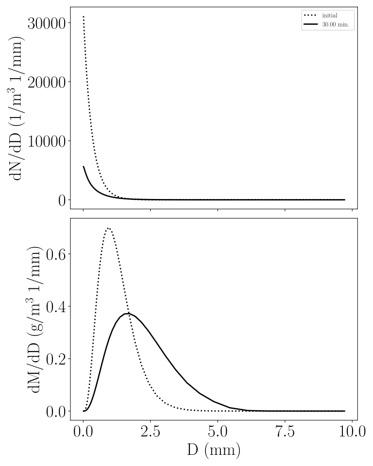
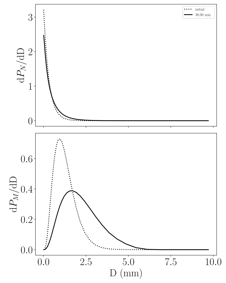
The number distribution function becomes a lot lower at \(30\) minutes due to collision-coalescence which rapidly decreases the number of raindrops with time. We can better compare the initial and final number distribution functions by using normbin=True which normalizes the number (mass) distribution by the total number (mass)

rain_box.plot_dists(-1,x_axis='size',xscale='linear',yscale='linear',distscale='linear',normbin=True)

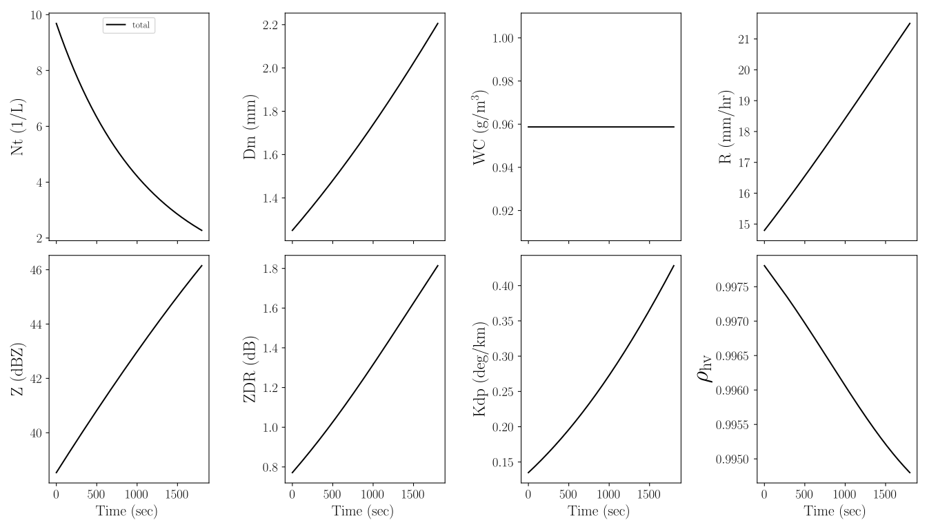
We can also look at the timeseries of the moments by using the plot_moments_radar() method:

rain_box.plot_moments_radar()

Notice that the liquid water content is constant throughout whereas the other variables increase or decrease approximately with generalized power-law behaviors.

Steady-state mode

Now we’ll replicate the box model run in the steady-state mode. To run the model as a steady-state model we can simply change a few of the inputs to the spectral_1d() initialization. In particular, we’ll use tmax=0 to indicate that we aren’t using the time domain at all (this indicates to BinMod1D that the steady-state mode is what we want) and we’ll set up the height domain by specifying the height grid spacing as dz=20. and the top and bottom heights as ztop=3000. and zbot=0. where each variable is in meters.

rain_SS = spectral_1d(sbin=2,bins=60,D1=0.01,tmax=0.,dz=20.,ztop=3000.,zbot=0.,Nt0=10.,Dm0=1.25,mu0=0.,habit_params=['rain'],ptype='rain',kernel='Hydro',Ecol=1.0,Es=0.2,radar=True,dist_var='size')
rain_SS.run()

Now we can plot the distributions as before to get a sense for what the final distributions look like. We can use the plot_dist() like before. plot_dists() can plot any time or height index using the tind or hind parameters. By default, the function plots the final distribution (i.e., tind=hind=-1) so we can just call the method like before without any arguments.

rain_SS.plot_dists(x_axis='size')

We can also reuse the plot_moments_radar() method to plot the steady-state height profiles for all variables

rain_SS.plot_moments_radar()

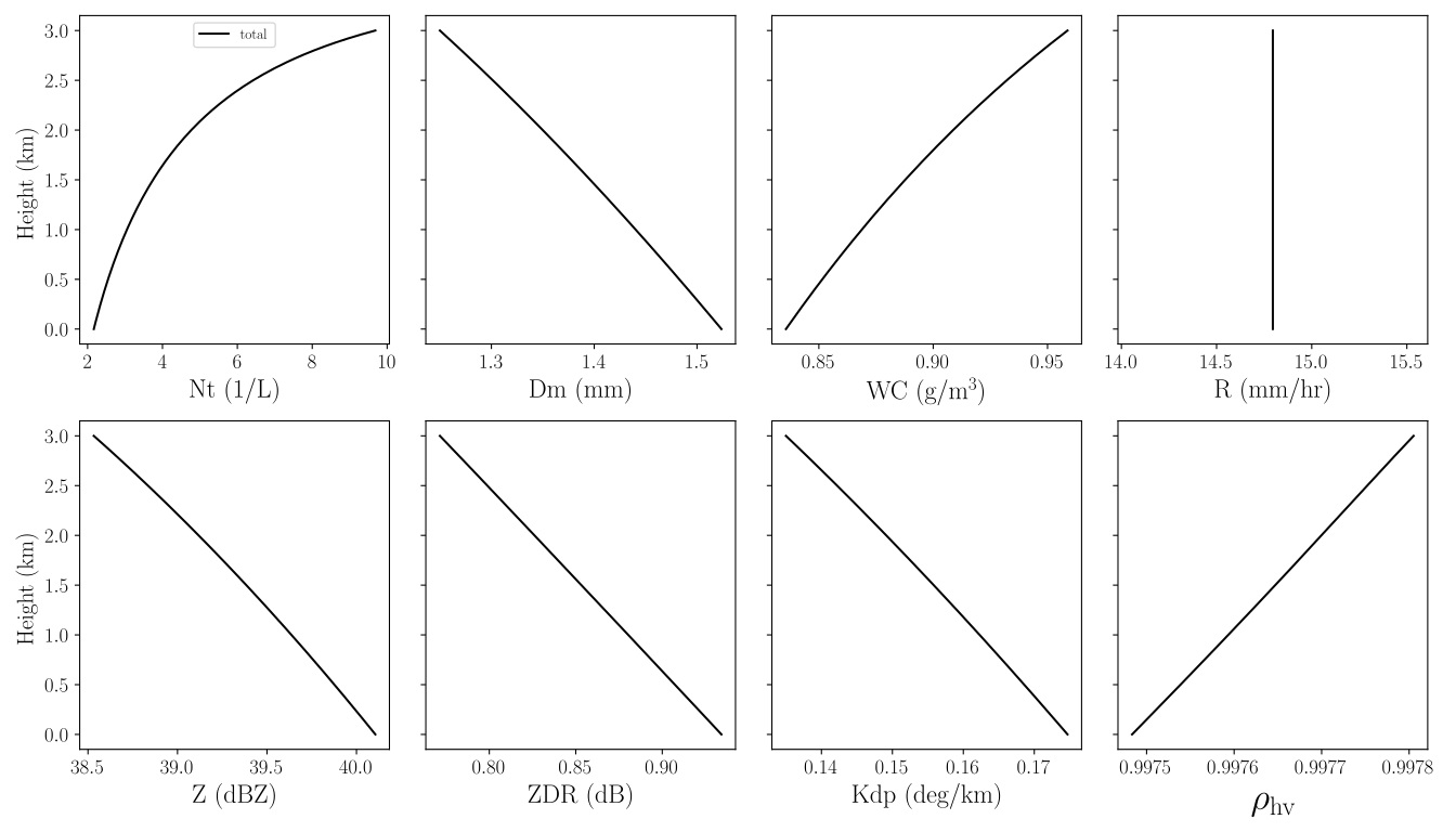
Notice that the mass flux, instead of the total mass, is conserved for all heights. Other variables decrease or increase in a generalized power-law-like way.

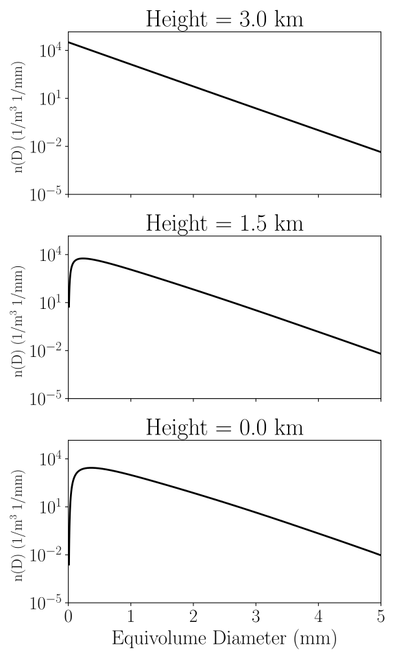
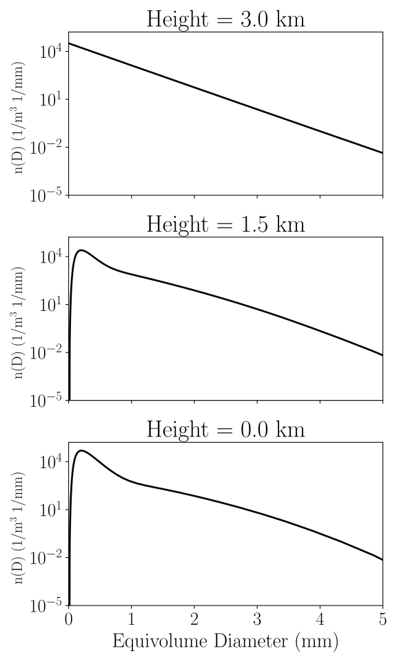
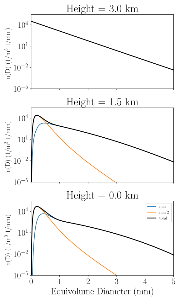
We can see the evolution of the particle size distributions with height by using the plot_dists_height() method. We’ll create a figure with 3 subpanels where we’ll plot the size distribution at \(3.0\) km, \(1.5\) km, and \(0\) km. To do this, we’ll use the dz input which specifies the dz spacing for each subplots between ztop and zbot.

rain_SS.plot_dists_height(dz=1.5)

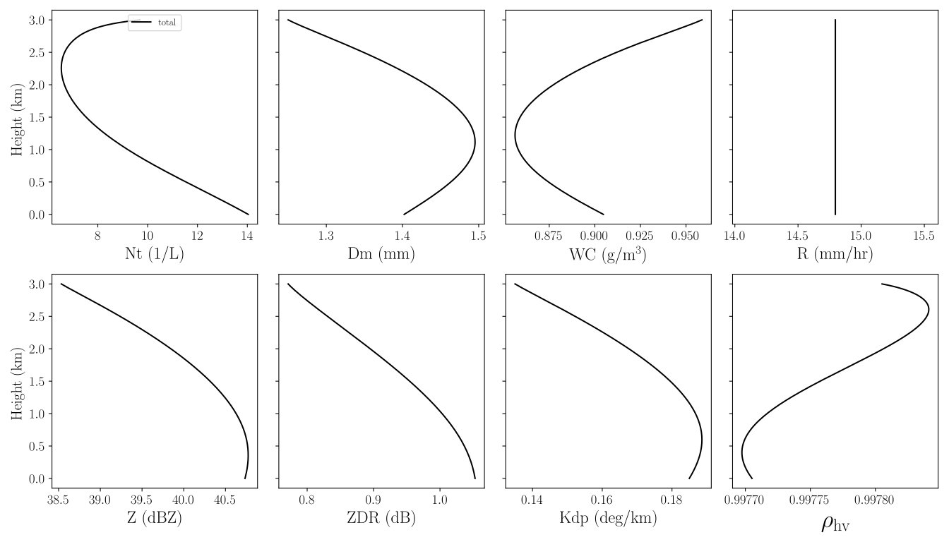
Now let’s try to incorporate breakup. We’ll set the breakup efficiency to \(0.035\) and we’ll raise the coalescence efficiency to \(0.8\) so that we can better see the effects of combined coalescence and breakup. We’ll also choose a lognormal distribution to represent fragments.

rain_breakup_SS = spectral_1d(sbin=2,bins=60,D1=0.01,tmax=0.,dz=20.,ztop=3000.,zbot=0.,Nt0=10.,Dm0=1.25,mu0=0.,habit_params=['rain'],frag_dist='LGN',ptype='rain',kernel='Hydro',Ecol=1.0,Es=0.8,Eb=0.035,radar=True,dist_var='size')
rain_breakup_SS.run()

Now let’s plot the resulting moments and radar variables as well as the same distribution plot as before with height

rain_breakup_SS.plot_moments_radar()
rain_breakup_SS.plot_dists_height(dz=1.5)

Full time/height mode (1D Column Model)

Finally, let’s do a full 1D model run with both coalescence and breakup turned on. To initialize a full 1D column model simulation, users just need to modify both the time (tmax) and top and bottom (ztop and zbot) input values. Let’s use the same tmax parameter (i.e., 30 minute simulation) along with the same height grid as in the steady-state example. We’ll also fix the top boundary conditon with boundary='fixed' in order for the model approach a steady-state solution after a sufficiently long period of time. Note that BinMod1D uses the Numba just-in-time (JIT) functionality which will parallelize calculations if users have multiple CPUs. Therefore, even this simulation will not take very long on most modern PCs.

rain_breakup_full = spectral_1d(sbin=2,bins=60,D1=0.01,dt=2,tmax=1800.,dz=20.,ztop=3000.,zbot=0.,Nt0=10.,Dm0=1.25,mu0=0.,habit_params=['rain'],frag_dist='LGN',ptype='rain',kernel='Hydro',boundary='fixed',Ecol=1.0,Es=0.8,Eb=0.035,radar=True,dist_var='size')
rain_breakup_full.run()

Now we can plot the full time/height reflectivity profile by using the plot_time_height() method. Reflectivity is plotted by default so we just need to call the function with no arguments.

rain_breakup_full.plot_time_height()

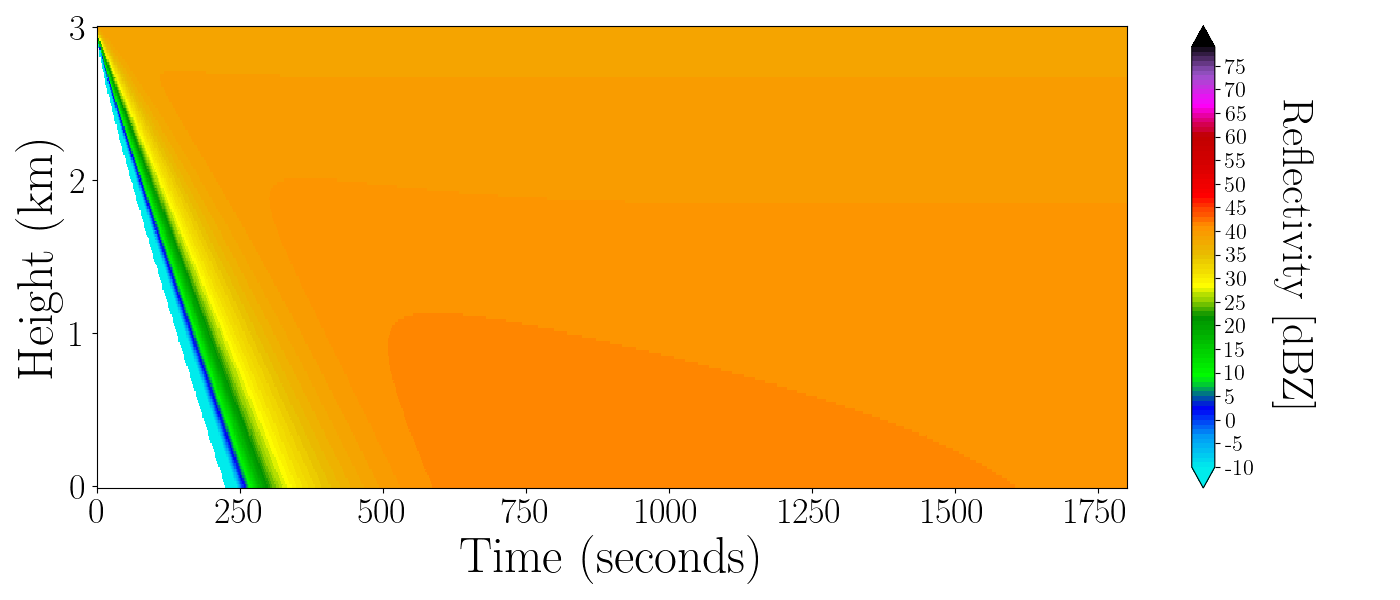
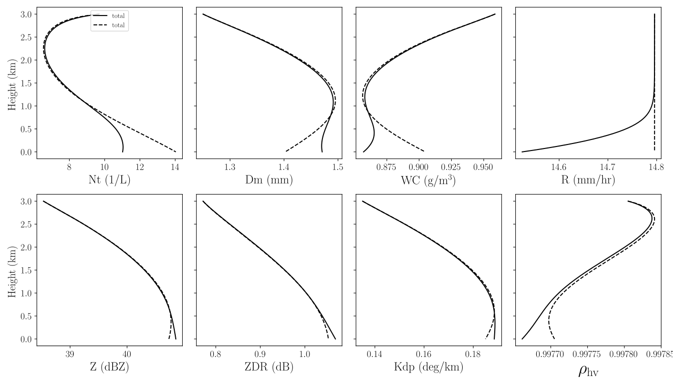
This simulation shows a rapid increase in simulated radar reflectivity toward the ground during the initial rain evolution due to rapid size sorting of large drops sedimenting and then a leveling off of reflectivity afterward in a quasi-steady state. We can use plot_moments_radar() to directly overlay the height profiles of the distribution and radar variables at \(30\) minutes with the steady-state solution from before. To do this, we first return the pyplot figure and axis when plotting the full 1D results. Then, we can use this axis handle as an input to the steady-state plotting. We can also use pyplot keyword arguments directly in plot_moments_radar() in order to modify line styles and other properites. Let’s set linestyle='--' when we plot the steady-state solution. This will plot the steady-state profiles with a dashed line whereas the full 1D column model will be plotted as a solid line.

fig, ax = rain_breakup_full.plot_moments_radar()
rain_breakup_SS.plot_moments_radar(ax=ax,linestyle='--')

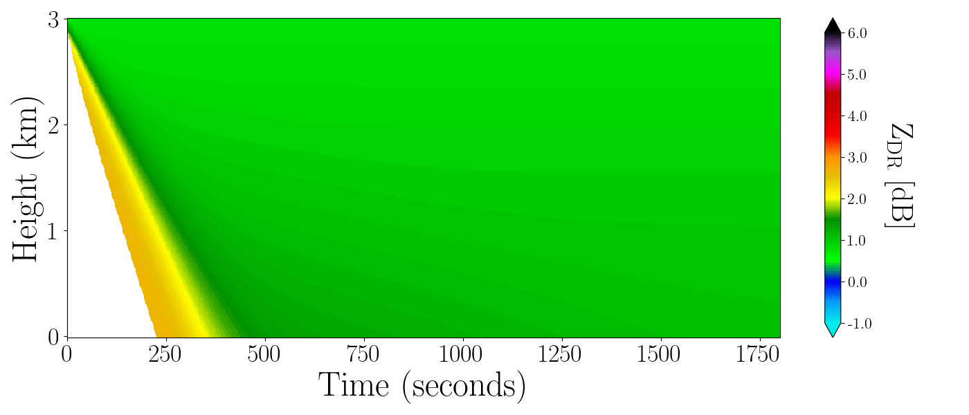
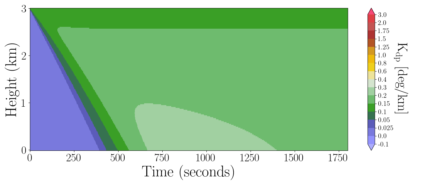
Finally we can plot the time/height profiles of the other radar variables using the var input parameter. If radar=True in the spectral_1d() object then users can plot any of the following variables: var=Z, var=ZDR, var=KDP, or var=RHOHV. Users can also plot any of the bulk microphysical properties as well (i.e., var='Nt, var=Dm, var=WC, var=R). Let’s plot differential reflecivity \(Z_{\mathrm{DR}}\) and specific differential phase \(K_{\mathrm{dp}}\)

rain_breakup_full.plot_time_height(var='ZDR')
rain_breakup_full.plot_time_height(var='KDP')

Customizing the model

Handling multiple distributions

BinMod1d can easily incorporate as many distributions as users want. To specify multiple distributions, users can use the habit_params input parameter. The habit_params parameter is a list of strings where each string dictates the type of habit that represents each distribution (e.g., ['snow','fragments']). Therefore, the length of the habit_params indicates the number of requested distributions. The individual strings represent the dictionary that’s used to determine the distributions properties (see the following section). Users can then specify which distribution receives coalesced particles by using the cc_dest parameter (value of 1 signifies the first distribution). Similarly, the br_dest determines the location of breakup (fragmented) particles. 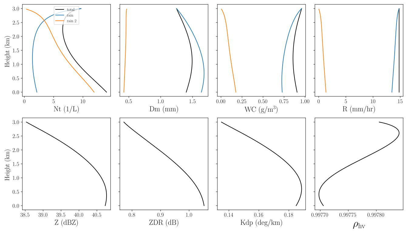Here, let’s keep the coalesced particles with the same distribution as the initial distribution but we’ll put the fragmented particles in a second distribution. Let’s use the steady-state coalescence/breakup example from before.

rain_breakup_SS_2cat = spectral_1d(sbin=2,bins=60,D1=0.01,tmax=0.,dz=20.,ztop=3000.,zbot=0.,Nt0=10.,Dm0=1.25,mu0=0.,habit_params=['rain','rain'],frag_dist='LGN',cc_dest=1,br_dest=2,ptype='rain',kernel='Hydro',Ecol=1.0,Es=0.8,Eb=0.035,radar=True,dist_var='size')
rain_breakup_SS_2cat.run()

We’ll use the plot_habits input parameter in the plots to specify that we want to see the individual distributions as well as the combined distribution variables.

rain_breakup_SS_2cat.plot_moments_radar(plot_habits=True)
rain_breakup_SS_2cat.plot_dists_height(dz=1.5,plot_habits=True)

Using custom distribution and habit parameters

spectral_1d() can specify each distribution’s initial particle size (mass) distribution, habit parameters, and fragment parameters through optional input parameters. There are six different possible methods for specifying the initial binned number and mass of each distributions using the init_method input parameter:

1. init_method='gamma'

Specifies an initial gamma distribution using the additional parameters: Nt0, Dm0, mu0, and gam_norm. Here, gam_norm specifies whether the normalized version of the gamma distribution is to be used (this, for example, is used in the BM1D_analytical_examples.ipyn jupyter notebook in order to compare the results with known analytical solutions).

2. init_method='analytical'

Users will use this input along with func_nD to specify the initial distribution where func_nD is an analytical lambda function (e.g., func_nD = lambda D: 10.*np.exp(-D)).

3. init_method='empirical

Users will use this input along with edges and nD where edges is a numpy array of size or mass bin edges determined by the var_dist parameter and nD is a numpy array of the number distribution function (in units of \(\mathrm{L}^{-1}\, \mathrm{mm}^{-1}\)) evaluated at each bin midpoint.

4. init_method='emprical_counts'

This is the same as init_method='empirical' with the exception that users pass in the bin counts (with input counts) rather than the number distribution function evaluated at the midpoint for the input of edges.

5. init_method='direct'

Users will use Mbins and/or Nbins and edges to directly determine the PSD. User’s values are then regridded onto the sbin bins geometric grid.

6. init_method='empty'

The distribution has no initial mass or number. This is typically how secondary category distributions are first initialized.

By default, BinMod1D has three example habit distributions with predetermined values: 'rain', 'snow', and 'fragments'. These dictionaries are available from the binmod1d.habits module.

from binmod1d.habits import habits, fragments
habits()

{'rain': {'arho': 1.0,
  'brho': 0.0,
  'av': 3.78,
  'bv': 0.67,
  'ar': 1.0,
  'br': 0.0,
  'sig': 10.0,
  'am': 0.0005235987755982988,
  'bm': 3.0},
 'snow': {'arho': 0.2,
  'brho': 1.0,
  'av': 0.8,
  'bv': 0.14,
  'ar': 0.6,
  'br': 0.0,
  'sig': 0.0,
  'am': 0.00010471975511965977,
  'bm': 2.0},
 'fragments': {'arho': 0.6,
  'brho': 0.0,
  'av': 0.8,
  'bv': 0.14,
  'ar': 0.8,
  'br': 0.0,
  'sig': 20.0,
  'am': 0.00031415926535897925,
  'bm': 3.0}}

Here, arho and brho represent the density-size power-law relation (\(\rho (D) = \alpha_{\rho} D^{-\beta_{\rho}}\)), av and bv represent the fallspeed-size power-law relation (\(v_{t}(D) = a_{v} D^{b_{v}}\)), ar and br represent the spheroidal aspect ratio-size power-law relation (\(\varphi (D)= a_{r} D^{br}\)), sig is the two-dimensional Gaussian orientation standard deviation parameter in degrees (see Ryzhkov et al. (2011)) where sig=0 is horizontally oriented and sig=40 is chaotically oriented, and am and bm are the mass-dimensional power-law parameters (\(m(D) = \alpha_{m} D^{\beta_{m}}\)). Users only need to modify the habit_params input parameter to spectral_1d().

For example, we can create a new habit dictionary for ice aggregates using the “Aggregates of densely rimed radiating assemblages of dendrites or dendrites” category from table 1 of Locatelli and Hobbs (1974)

 agg_dict = {'agg':{'av': 0.79,
   'bv': 0.27,
   'ar': 0.6,
   'br': 0.0,
   'sig': 10.0,
   'am': 3.7e-05,
   'bm': 1.9}}

Then the dictionary can be passed into the spectral_1d() initialization call

s_agg = spectral_1d(habit_params=agg_dict)

Note that users only need to specify either am and bm or arho and brho; the mass or density parameters will be determined by either pair. Users can also combine their own custom habit dictionaries with the preset dictionaries from the habits.py module. In this way, each list element will be treated as a separate category.

s_agg = spectral_1d(habit_params=['snow',agg_dict],cc_dest=2)

Users can also implement their own fallspeed-size and aspect ratio-isze parameterizations as well. To do this, users use either aspect_ratio= lambda d: aspect_ratio(d) or vt=lambda d: fallspeed(d) as inputs to spectral_1d() where aspect_ratio(d) and fallspeed(d) are custom functions that users would like to use to specify the aspect ratio-size and/or fallspeed-size relationships.

Users can similarly modify the fragment distribution using the frag_dist input parameter. Default fragment size distributions are provided in the binmod1d.habits.fragments function for an exponential (frag_dist='exp'), a gamma (frag_dist='gamma'), and lognormal (frag_dist='LGN') distribution. Additionally, users can use the Straub et al. (2010) multimodal fragment distribution as well with (frag_dist='Straub'). Therefore, users can either specify one of these distributions when initializing spectral_1d()

s_frag = spectral_1d(frag_dist='LGN',habit_params=['rain','rain'],cc_dest=1,br_dest=2)

or users can create their own distribution functions using the same dictionary structure. For example, the lognormal fragment distribution has the following default dictionary:

        {'dist': 'LGN',
         'var': 'size',
         'Df_med': 0.25,
         'Df_mode': 0.2,
         'cdf_bounds': (0.5, 0.95),
         'parent_cutoff':0.,
         'd_start': np.float64(0.25),
         'd_end': np.float64(0.5437328654539426),
         'func': <function binmod1d.habits.fragments.<locals>.<lambda>(n, c, pi, pj)>}

Here, dist is the name of the distribution, var is whether the fragment distribution is defined in terms of mass ('mass') or size ('size'), ‘Df_med’ and ‘Df_mode’ are the lognormal distribution parameters, cdf_bounds are the requested percentile bounds of the lognormal distribution where the distribution will become active. The d_start and d_end parameters correspond to the 50% and 95% percentiles where d<d_start will not be active, d_start<d<d_end will ramp from \(0\) to \(E_{\mathrm{b}}\), and d>d_end will have \(E_{\mathrm{b}}\). The lambda function func are the output conditional bin-wise moments of the defined fragment distribution

\[ P_{k}^{n}(\mathbf{x_{i}},\mathbf{x_{j}}) = \int\limits_{m=m_{k}}^{m_{k+1}} m^{n} P(m|\mathbf{x_{i}},\mathbf{x_{j}})\, dm, \qquad \texttt{var = "mass"} \]

or

\[ P_{k}^{n}(\mathbf{x_{i}},\mathbf{x_{j}}) = \int\limits_{D=D_{k}}^{D_{k+1}} D^{n} P(D|\mathbf{x_{i}},\mathbf{x_{j}})\, dD, \qquad \texttt{var = "size"} \]

Users who want to create their own fragment distributions simply need to structure their lambda function as follows:

FOR var = 'size'

    func = lambda n, c, pi, pj: dist_int(*params,n,c.d1,c.d2)

FOR var = 'mass'

    func = lambda n, c, pi, pj: dist_int(*params,n,c.xi1,c.xi2)

where c corresponds to the fragment distribution whereas pi and pj correspond to the i and j distributions of the parent interacting bins.

Note, for marginal distributions which use a static (yet truncated) distribution (as with the examples shown here), pi and pj do not need to be used in the lambda function but still need to be inputs. For conditional fragment distributions of the form \(P(m|x,y)\), users can use the pi and pj object inputs to structure the conditional nature of the multivariate distribution function. For example, if the conditional distribution depends upon the i and j bin midpoint fall speeds, then the lambda function structure might be something like:

    func = lambda n, c, pi, pj: dist_int(n,c.d1,c.d2,pi.vt,pj.vt). 

Reading and writing netcdf outputs

After users run their model with run(), they can easily save their model results using the write_netcdf() method.

Let’s use the first steady-state Jupyter notebook test to demonstrate this.

from binmod1d.spectral_model import spectral_1d
s3_SS = spectral_1d(sbin=3,bins=160,D1=0.001,tmax=0.,Nt0=15.,Dm0=0.8,mu0=0.,dz=10.0,ztop=1000.,zbot=0.,habit_params=['rain'],ptype='rain',kernel='Hydro',Ecol=1.0,Es=0.8,radar=True,dist_var='size')
s3_SS.run()

Now users can write a netcdf file with all the simulated distribution function parameters to a file by simply running write_netcdf(filename) where filename is the full path to the directory and filename where they would like to save the netcdf file

s3_SS.write_netcdf('C://Users/username/Documents/BinMod1D/s3_SS.nc')

Loading previous model run netcdf files is trivial. To do so, just use the load input parameter in the spectral_1d() class without any other inputs.

s3_SS_load = spectral_1d(load='C://Users/username/Documents/BinMod1D/s3_SS.nc')

spectral_1d() will read the 4D binned mass (or mass and number if moments=2) distribution for all output times and heights, any input parameters that were used during the initialization, and will recalculate the linear subgrid distribution parameters, and bulk microphysical and radar (if radar=True was specified during initialization) variables.

References

Locatelli, J. D. and P. V. Hobbs, 1974: Fall speeds and masses of solid precipitation particles, J. Geophys. Res., 79, 2185–2197, https://doi.org/10.1029/JC079i015p02185

Ryzhkov, A., Pinsky, M., Pokrovsky, A., and Khain, A., 2011: Polarimetric radar observation operator for a cloud model with spectral microphysics, J. Appl. Meteor. Climatol., 50, 873–894, https://doi.org/10.1175/2010JAMC2363.1

Straub, W., Beheng, K. D., Seifert, A. Schlottke, J., and Weigand, B., 2010: Numerical investigation of collision-induced breakup of raindrops. Part II: Parameterizations of coalescence efficiencies and fragment size distributions, J. Atmos. Sci., 46, 576–588, https://doi.org/10.1175/2009JAS3175.1